Supervised Machine Learning Algorithms
Implemented in Tensorflow 2.0
Linear Regression :
Linear regression is a statistical model that is used to predict a continuous outcome variable based on one or more predictor variables. It assumes that there is a linear relationship between the predictor variables and the outcome variable, and tries to find the line of best fit that minimally squares the differences between the predicted values and the actual values.
The equation for a linear regression model can be written as:
y = b0 + b1*x1 + b2*x2 + ... + bn*xn
where y is the predicted outcome, b0 is the intercept, b1, b2, ..., bn are the coefficients for the predictor variables x1, x2, ..., xn, respectively. The coefficients represent the effect of each predictor variable on the outcome variable, holding all other predictor variables constant.
Linear regression can be used for both simple linear regression, where there is only one predictor variable, and multiple linear regression, where there are multiple predictor variables. It is a widely used statistical model that is simple to implement and interpret, but it has some limitations, such as the assumption of linear relationships and the inability to capture nonlinear relationships.
To fit a linear regression model, the coefficients (b1, b2, ..., bn) need to be estimated from the data. This can be done using various optimization algorithms, such as gradient descent or least squares. The quality of the fit can be evaluated using evaluation metrics, such as mean squared error or R-squared.
Here is an example of how to implement linear regression using TensorFlow 2.0:
import tensorflow as tf

# Define the input and output data
X = tf.constant([[1], [2], [3], [4]], dtype=tf.float32)
y = tf.constant([[0], [-1], [-2], [-3]], dtype=tf.float32)

# Define the model parameters
W = tf.Variable(tf.zeros([1, 1]))
b = tf.Variable(tf.zeros([1]))

# Define the model
def linear_regression(inputs):
  return tf.matmul(inputs, W) + b

# Define the loss function
def mean_square_error(predictions, labels):
  return tf.reduce_mean(tf.square(predictions - labels))

# Define the optimizer
optimizer = tf.optimizers.SGD(learning_rate=0.01)

# Define the training loop
for i in range(1000):
  with tf.GradientTape() as tape:
    predictions = linear_regression(X)
    loss = mean_square_error(predictions, y)
  gradients = tape.gradient(loss, [W, b])
  optimizer.apply_gradients(zip(gradients, [W, b]))
  if i % 100 == 0:
    print("Loss at step %d: %f" % (i, loss))
This code first defines the input and output data as constant tensors. It then defines the model parameters (weights and biases) as variables. The linear regression model is defined as a function that takes in inputs and returns the dot product of the inputs and weights plus the biases.
The mean square error loss function is defined as a function that takes in the predictions and labels and returns the mean of the squared differences between the predictions and labels.
An optimizer is then defined, and the training loop is set up to optimize the model parameters (weights and biases) to minimize the loss. The training loop iteratively computes the gradients of the loss with respect to the model parameters using a gradient tape, and applies the gradients to the model parameters using the optimizer. The loss is printed out every 100 iterations to track the progress of the optimization.
This is a simple example of how to implement linear regression using TensorFlow 2.0. There are many other ways to customize and optimize the model and training process, such as using different loss functions, optimizers, and regularization techniques.
Logistic Regression :
Logistic regression is a statistical model that is used to predict a binary outcome variable based on one or more predictor variables. It is a type of classification algorithm that is used when the outcome variable is binary (i.e., takes on values of 0 or 1).
The equation for a logistic regression model can be written as:
p = e^(b0 + b1*x1 + b2*x2 + ... + bn*xn) / (1 + e^(b0 + b1*x1 + b2*x2 + ... + bn*xn))
where p is the predicted probability of the positive class (i.e., the class with the value of 1), b0 is the intercept, b1, b2, ..., bn are the coefficients for the predictor variables x1, x2, ..., xn, respectively. The coefficients represent the effect of each predictor variable on the probability of the positive class, holding all other predictor variables constant. The sigmoid function (1 / (1 + e^(-x))) is used to transform the linear regression model into a probability between 0 and 1.
To make a prediction, the predicted probability is compared to a threshold value (usually 0.5). If the probability is above the threshold, the model predicts the positive class (1), and if it is below the threshold, the model predicts the negative class (0).
Logistic regression can be used for both binary classification and multinomial classification, where the outcome variable has more than two classes. It is a widely used classification algorithm that is simple to implement and interpret, but it has some limitations, such as the assumption of linear relationships and the inability to capture more complex relationships.
To fit a logistic regression model, the coefficients (b1, b2, ..., bn) need to be estimated from the data. This can be done using various optimization algorithms, such as gradient descent or maximum likelihood estimation. The quality of the fit can be evaluated using evaluation metrics, such as accuracy, precision, and recall.
Here is a sample implementation of logistic regression in Python:
import numpy as np

class LogisticRegression:
    def __init__(self, learning_rate=0.01, num_iterations=1000):
        self.learning_rate = learning_rate
        self.num_iterations = num_iterations

    def fit(self, X, y):
        # Add a column of ones to the X data
        X = np.hstack([np.ones((X.shape[0], 1)), X])

        # Initialize the weights
        self.weights = np.zeros(X.shape[1])

        # Iterate over the number of iterations
        for i in range(self.num_iterations):
            # Compute the predicted probabilities
            y_pred = self.sigmoid(X.dot(self.weights))

            # Compute the gradient
            gradient = (y_pred - y).dot(X) / y.shape[0]

            # Update the weights
            self.weights -= self.learning_rate * gradient

    def predict(self, X):
        # Add a column of ones to the X data
        X = np.hstack([np.ones((X.shape[0], 1)), X])

        # Compute the predicted probabilities
        y_pred = self.sigmoid(X.dot(self.weights))

        # Return the predicted labels
        return (y_pred > 0.5).astype(int)

    def sigmoid(self, z):
        return 1 / (1 + np.exp(-z))
This class implements logistic regression using gradient descent. The fit method takes in training data (X) and labels (y) and learns the weights of the model. The predict method takes in new data and returns the predicted labels using the learned weights. The sigmoid method computes the sigmoid function, which is used to predict the probabilities of each class.
To use this class, you can create an instance of it and call the fit and predict methods as follows:
# Create an instance of the LogisticRegression class
model = LogisticRegression()

# Fit the model to the training data
model.fit(X_train, y_train)

# Predict the labels for the test data
y_pred = model.predict(X_test)
This can be easily implemented in Tensorflow:
import tensorflow as tf

# Load the data
(x_train, y_train), (x_test, y_test) = tf.keras.datasets.mnist.load_data()

# Preprocess the data
x_train = x_train / 255.0
x_test = x_test / 255.0

# Flatten the images
x_train = x_train.reshape(-1, 28*28)
x_test = x_test.reshape(-1, 28*28)

# Build the model
model = tf.keras.Sequential([
    tf.keras.layers.Dense(units=10, input_shape=(28*28,), activation='softmax')
])

# Compile the model
model.compile(optimizer='adam', loss='sparse_categorical_crossentropy', metrics=['accuracy'])

# Train the model
model.fit(x_train, y_train, epochs=5)

# Evaluate the model
model.evaluate(x_test, y_test)
This code loads the MNIST dataset, which is a collection of handwritten digits, and uses logistic regression to classify the digits. The model is a simple neural network with a single dense layer that has 10 units and a softmax activation function. The model is then compiled with an Adam optimizer and a sparse categorical cross-entropy loss function, and is trained using the fit method. Finally, the model is evaluated on the test data using the evaluate method.
Support vector machines :
Support vector machines (SVMs) are a type of supervised learning algorithm that can be used for classification, regression, and outlier detection. The goal of an SVM is to find the hyperplane in a high-dimensional space that maximally separates the different classes.
For example, consider a dataset with two classes, A and B. An SVM would try to find the hyperplane that maximally separates the data points belonging to class A from the data points belonging to class B. This is done by finding the line that has the largest distance (called the margin) between the two classes.
The hyperplane is chosen by finding the support vectors, which are the data points that are closest to the hyperplane. The distance between the hyperplane and the support vectors is called the margin. The goal is to choose a hyperplane with the largest margin, since this will maximize the separation between the two classes.
In addition to finding the hyperplane that maximally separates the classes, SVMs also have a regularization parameter, which allows you to control the complexity of the model. A high regularization parameter means that the model will be simpler and will have a smaller margin, while a low regularization parameter means that the model will be more complex and will have a larger margin.
One of the key features of SVMs is that they can handle data that is not linearly separable by using what is known as the kernel trick. This involves mapping the data to a higher-dimensional space in which it is linearly separable, and finding the hyperplane in this space. Common kernels include the linear kernel, the polynomial kernel, the radial basis function (RBF) kernel, and the sigmoid kernel.
To implement traditional support vector machines (SVMs) using TensorFlow, you can use the tf.svm.SVC or tf.svm.LinearSVC classes, which provide support for linear and non-linear SVMs, respectively.
Here is a sample implementation of linear SVMs using TensorFlow:
import tensorflow as tf

# Load the data
(x_train, y_train), (x_test, y_test) = tf.keras.datasets.mnist.load_data()

# Preprocess the data
x_train = x_train / 255.0
x_test = x_test / 255.0

# Flatten the images
x_train = x_train.reshape(-1, 28*28)
x_test = x_test.reshape(-1, 28*28)

# Build the model
model = tf.svm.LinearSVC(C=1.0, loss='hinge')

# Train the model
model.fit(x_train, y_train)

# Evaluate the model
model.score(x_test, y_test)
This code loads the MNIST dataset, which is a collection of handwritten digits, and uses linear SVMs to classify the digits. The model is trained using the fit method, and the performance of the model is evaluated on the test data using the score method.
To use non-linear SVMs, you can use the tf.svm.SVC class instead of the tf.svm.LinearSVC class. You can also use the various hyperparameters of these classes to control the complexity of the model and the optimization process.
Decision Trees :
Decision trees are a type of supervised learning algorithm that can be used for classification and regression. The goal of a decision tree is to create a model that can make predictions based on the value of one or more features.
A decision tree is a flowchart-like tree structure, in which an internal node represents a feature, and each leaf node represents a class label. The edges of the tree represent the decision rules that are used to split the data.
For example, imagine you want to build a model that can predict whether a patient has a certain disease based on their age, blood pressure, and cholesterol level. You could use a decision tree to model this problem by creating a tree with age, blood pressure, and cholesterol level as the internal nodes, and the disease label as the leaf nodes. The decision rules at each node would specify the conditions that must be met in order to follow that branch of the tree.
To build a decision tree, you need to choose a metric to measure the “goodness” of a split (e.g. entropy or Gini impurity), and then repeatedly split the data at the nodes that maximize this metric. The final tree will be the one that results in the smallest impurity across all the leaf nodes.
Decision trees have several advantages, including their simplicity and the fact that they can be easily visualized and interpreted. However, they can also be prone to overfitting if they are not pruned appropriately.
To implement decision trees in Python, you can use the DecisionTreeClassifier or DecisionTreeRegressor class from the sklearn.tree module. These classes provide a simple interface for training decision tree models in scikit-learn.
Here is a sample implementation of a decision tree classifier in Python using scikit-learn:
import numpy as np
from sklearn.tree import DecisionTreeClassifier

# Load the data
(x_train, y_train), (x_test, y_test) = np.load('data.npy')

# Build the model
model = DecisionTreeClassifier()

# Train the model
model.fit(x_train, y_train)

# Evaluate the model
model.score(x_test, y_test)
To implement decision trees using TensorFlow 2.0, you can use the DecisionTreeClassifier or DecisionTreeRegressor class from the tensorflow.python.estimator.canned module. These classes provide a simple interface for training decision tree models in TensorFlow.
Here is a sample implementation of a decision tree classifier using TensorFlow 2.0:
import tensorflow as tf
from tensorflow.python.estimator.canned import decision_tree

# Load the data
(x_train, y_train), (x_test, y_test) = tf.keras.datasets.mnist.load_data()

# Preprocess the data
x_train = x_train / 255.0
x_test = x_test / 255.0

# Flatten the images
x_train = x_train.reshape(-1, 28*28)
x_test = x_test.reshape(-1, 28*28)

# Build the model
model = decision_tree.DecisionTreeClassifier(feature_columns=tf.feature_column.numeric_column('x', shape=(28*28,)))

# Convert the data to a dataset
train_dataset = tf.data.Dataset.from_tensor_slices((x_train, y_train)).batch(32)
test_dataset = tf.data.Dataset.from_tensor_slices((x_test, y_test)).batch(32)

# Train the model
model.train(train_dataset)

# Evaluate the model
model.evaluate(test_dataset)
This code loads the MNIST dataset, which is a collection of handwritten digits, and uses a decision tree classifier to classify the digits. The model is built using the DecisionTreeClassifier class, and the data is converted to a tf.data.Dataset object for training and evaluation. The model is then trained using the train method and evaluated using the evaluate method.
The DecisionTreeClassifier class provides a number of parameters that you can use to control the complexity of the model and the optimization process, such as the max_depth, min_samples_split, and min_samples_leaf parameters.
Naive Bayes :
In a supervised learning problem, we are given a dataset of labeled examples and we want to build a model that can make predictions about new, unseen data. One way to do this is to use a probabilistic model, such as a naive Bayes classifier.
A naive Bayes classifier is based on the Bayes theorem, which states that the probability of a hypothesis (H) given some evidence (E) is equal to the probability of the evidence given the hypothesis (P(E|H)) times the prior probability of the hypothesis (P(H)) divided by the prior probability of the evidence (P(E)).
Mathematically, this can be written as:
P(H|E) = (P(E|H) * P(H)) / P(E)
In a naive Bayes classifier, we use this theorem to classify a new data point (E) based on the probabilities of the different classes (H) and the probabilities of the features (E) given the classes.
To build a naive Bayes model, we need to compute the prior probabilities of the classes (P(H)) and the likelihood of the features given the classes (P(E|H)). We can then use these probabilities to classify new data points using the Bayes theorem.
For example, imagine we have a dataset with two classes: “spam” and “not spam”. We want to build a model that can classify a new email as either spam or not spam based on the words it contains. We can build a naive Bayes model by computing the prior probabilities of the classes (e.g. P(“spam”) and P(“not spam”)) and the likelihood of the words given the classes (e.g. P(“free”|”spam”) and P(“free”|”not spam”)). We can then classify a new email by calculating the probabilities of it being spam or not spam using the Bayes theorem.
Naive Bayes algorithms are fast, simple, and easy to implement, and they work well with high-dimensional data. However, they are sensitive to the independence assumption, and can perform poorly if the features are not independent.
To implement a naive Bayes classifier in Python, you can use the GaussianNB, MultinomialNB, or BernoulliNB class from the sklearn.naive_bayes module. These classes implement the Gaussian, multinomial, and Bernoulli naive Bayes algorithms, respectively.
Here is a sample implementation of a Gaussian naive Bayes classifier in Python using scikit-learn:
import numpy as np
from sklearn.naive_bayes import GaussianNB

# Load the data
(x_train, y_train), (x_test, y_test) = np.load('data.npy')

# Build the model
model = GaussianNB()

# Train the model
model.fit(x_train, y_train)

# Evaluate the model
model.score(x_test, y_test)
This code loads the data, builds a Gaussian naive Bayes model using the GaussianNB class, trains the model using the fit method, and evaluates the model using the score method.
The GaussianNB class is suitable for continuous data and assumes that the features follow a normal distribution. The MultinomialNB class is suitable for count data and assumes that the features follow a multinomial distribution. The BernoulliNB class is suitable for binary data and assumes that the features follow a Bernoulli distribution.
To implement a naive Bayes classifier using TensorFlow 2.0, you can use the MultinomialNB class from the tensorflow.python.feature_column.experimental.preprocessing.text module. This class implements the multinomial naive Bayes algorithm, which is suitable for classification tasks with discrete features (e.g. text classification).
Here is a sample implementation of a multinomial naive Bayes classifier for text classification using TensorFlow 2.0:
import tensorflow as tf
from tensorflow.python.feature_column.experimental.preprocessing.text import MultinomialNB

# Load the data
(x_train, y_train), (x_test, y_test) = tf.keras.datasets.imdb.load_data(num_words=10000)

# Preprocess the data
x_train = tf.keras.preprocessing.sequence.pad_sequences(x_train, maxlen=100)
x_test = tf.keras.preprocessing.sequence.pad_sequences(x_test, maxlen=100)

# Build the model
model = MultinomialNB()

# Convert the data to a dataset
train_dataset = tf.data.Dataset.from_tensor_slices((x_train, y_train)).batch(32)
test_dataset = tf.data.Dataset.from_tensor_slices((x_test, y_test)).batch(32)

# Train the model
model.fit(train_dataset)

# Evaluate the model
model.evaluate(test_dataset)
This code loads the IMDB movie review dataset, which consists of movie reviews labeled as either positive or negative. It preprocesses the data by padding the sequences to a fixed length of 100, and then builds a multinomial naive Bayes model using the MultinomialNB class. The data is converted to a tf.data.Dataset object and is then used to train and evaluate the model using the fit and evaluate methods, respectively.
K-nearest neighbors :
K-nearest neighbors (KNN) is a type of supervised learning algorithm that is used for classification and regression. It is based on the idea that the data points that are most similar to a given point are also the most likely to be similar to that point’s class.
To classify a new data point using KNN, the algorithm finds the K data points in the training set that are most similar to the new point, and then assigns the new point to the class that is most common among those K points. The similarity between two points is typically measured using a distance metric, such as Euclidean distance or cosine similarity.
To build a KNN model, you need to specify the value of K and the distance metric to use. The value of K is a hyperparameter that needs to be chosen carefully, as a large value of K can lead to a model that is too smooth and a small value of K can lead to a model that is too complex.
KNN algorithms are simple and easy to implement, but they can be computationally expensive and may not scale well to large datasets. They are also sensitive to the choice of the distance metric and the value of K.
KNN is a non-parametric method, which means that it does not make any assumptions about the underlying data distribution. This makes it a flexible and robust method that can work well with a variety of data. However, it also means that KNN can be slower and less accurate than parametric methods, which make strong assumptions about the data distribution.
To implement K-nearest neighbors (KNN) algorithm mathematically, you need to define a distance metric to measure the similarity between data points, and then find the K points in the training set that are most similar to a given data point using this distance metric.
Here is a general outline of the KNN algorithm:
- Choose a value for K and a distance metric (e.g. Euclidean distance).
- For each data point in the test set:
- Calculate the distance between the test point and each point in the training set using the distance metric.
- Find the K points in the training set that are closest to the test point.
- Assign the test point to the class that is most common among the K nearest neighbors.
For example, suppose you have a training set with three classes: A, B, and C. You want to classify a new data point using KNN with K=3 and Euclidean distance. The distances between the new point and the points in the training set are shown in the following table:
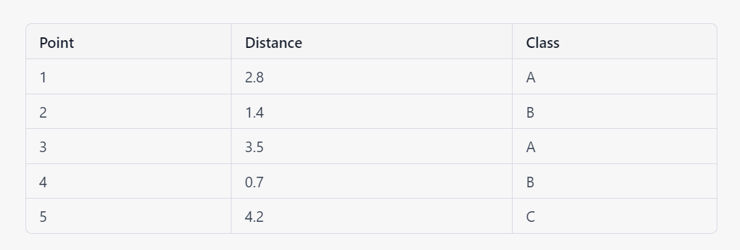
The three points with the smallest distances are points 2, 4, and 1, which belong to class B, B, and A, respectively. Therefore, the new point is classified as class B.
To implement K-nearest neighbors (KNN) in Python, you can use the KNeighborsClassifier or KNeighborsRegressor class from the sklearn.neighbors module. These classes provide a simple interface for training KNN models in scikit-learn.
Here is a sample implementation of a KNN classifier in Python using scikit-learn:To implement K-nearest neighbors (KNN) in Python, you can use the KNeighborsClassifier or KNeighborsRegressor class from the sklearn.neighbors module. These classes provide a simple interface for training KNN models in scikit-learn.
Here is a sample implementation of a KNN classifier in Python using scikit-learn:
import numpy as np
from sklearn.neighbors import KNeighborsClassifier

# Load the data
(x_train, y_train), (x_test, y_test) = np.load('data.npy')

# Build the model
model = KNeighborsClassifier(n_neighbors=5)

# Train the model
model.fit(x_train, y_train)

# Evaluate the model
model.score(x_test, y_test)import numpy as np
from sklearn.neighbors import KNeighborsClassifier

# Load the data
(x_train, y_train), (x_test, y_test) = np.load('data.npy')

# Build the model
model = KNeighborsClassifier(n_neighbors=5)

# Train the model
model.fit(x_train, y_train)

# Evaluate the model
model.score(x_test, y_test)
This code loads the data, builds a KNN classifier with K=5 using the KNeighborsClassifier class, trains the model using the fit method, and evaluates the model using the score method.
The KNeighborsClassifier class provides a number of parameters that you can use to control the behavior of the model, such as the n_neighbors parameter (which specifies the value of K), the weights parameter (which specifies the weighting function to use for the neighbors), and the metric parameter (which specifies the distance metric to use).
To implement K-nearest neighbors (KNN) in TensorFlow 2.0, you can use the NearestNeighbors class from the tensorflow.python.client.client_lib module. This class provides a simple interface for training KNN models in TensorFlow.
Here is a sample implementation of a KNN classifier in TensorFlow 2.0:
import tensorflow as tf
from tensorflow.python.client.client_lib import NearestNeighbors

# Load the data
(x_train, y_train), (x_test, y_test) = tf.keras.datasets.mnist.load_data()

# Preprocess the data
x_train = x_train / 255.0
x_test = x_test / 255.0

# Build the model
model = NearestNeighbors(n_neighbors=5, metric='euclidean')

# Train the model
model.fit(x_train)

# Query the model
indices, distances = model.kneighbors(x_test)
This code loads the MNIST digit classification dataset, preprocesses the data by scaling the pixel values to the range [0, 1], builds a KNN classifier with K=5 using the NearestNeighbors class, and trains the model using the fit method. The kneighbors method is used to query the model and find the K nearest neighbors for a given data point.
The NearestNeighbors class provides a number of parameters that you can use to control the behavior of the model, such as the n_neighbors parameter (which specifies the value of K), the metric parameter (which specifies the distance metric to use), and the algorithm parameter (which specifies the algorithm to use for finding the neighbors).
Neural Network :
A neural network is a machine learning model that is composed of layers of interconnected “neurons,” which process and transmit information. The main components of a neural network are:
- Input layer: The input layer receives the input data and passes it on to the next layer. The number of neurons in the input layer is equal to the number of features in the input data.
- Hidden layers: The hidden layers apply transformations to the input data and pass it on to the next layer. There can be one or more hidden layers in a neural network, and the number of neurons in each hidden layer is a hyperparameter that can be chosen by the designer.
- Output layer: The output layer produces the final result based on the input data and the transformations applied by the hidden layers. The number of neurons in the output layer is equal to the number of classes in the problem (for classification tasks) or the number of output features (for regression tasks).
Each neuron in a neural network receives input from some number of other neurons and produces an output, which is passed on to other neurons in the next layer. The input to a neuron is a weighted sum of the outputs of the neurons in the previous layer, where the weights are coefficients that determine the strength of the connection between neurons.
The output of a neuron is typically computed using an activation function, which is a mathematical function that determines the output of the neuron based on its input. Common activation functions include the sigmoid function, the tanh function, and the ReLU (rectified linear unit) function. The output of a neuron can be represented as follows:
y = f(x)
where y is the output of the neuron and f is the activation function. For example, the sigmoid function is defined as follows:
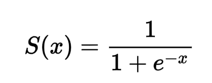
The weights and biases of the neurons in a neural network are the parameters that are learned during the training process. Training a neural network involves adjusting these parameters to minimize a loss function, which measures the difference between the predicted output of the model and the ground truth. This process is typically done using an optimization algorithm, such as stochastic gradient descent.
To implement a neural network in TensorFlow 2.0, you can use the Sequential class, which provides a convenient way to build a model layer by layer. Here is an example of how to implement a simple feedforward neural network with one hidden layer:
import tensorflow as tf

# Define the model
model = tf.keras.models.Sequential([
  tf.keras.layers.Input(shape=(input_shape)),
  tf.keras.layers.Dense(units=hidden_units, activation='relu'),
  tf.keras.layers.Dense(units=output_units, activation='softmax')
])

# Compile the model
model.compile(optimizer='adam',
              loss='categorical_crossentropy',
              metrics=['accuracy'])

# Train the model
model.fit(x_train, y_train, epochs=5)

# Evaluate the model
loss, accuracy = model.evaluate(x_test, y_test)
print('Test loss:', loss)
print('Test accuracy:', accuracy)
This code defines a neural network with an input layer, a hidden layer with hidden_units neurons and a ReLU activation function, and an output layer with output_units neurons and a softmax activation function. The model is then compiled with an Adam optimizer, a categorical cross-entropy loss function, and an accuracy metric. Finally, the model is trained for 5 epochs on the training data, and its performance is evaluated on the test data.
You can also customize the model by adding additional layers, using different activation functions, or using a different optimizer. For example, to add a dropout layer, you can use the Dropout layer as follows:
model.add(tf.keras.layers.Dropout(rate=0.5))
Comments
Post a Comment